Demo

import numpy as np
import scipy as sp
import scipy.sparse
import matplotlib.pyplot as plt
%matplotlib inline

from bayesbridge import BayesBridge, RegressionModel, RegressionCoefPrior
from simulate_data import simulate_design, simulate_outcome
from util import mcmc_summarizer

BayesBridge supports both dense (numpy array) and sparse (scipy sparse matrix) design matrices.

n_obs, n_pred = 10 ** 4, 10 ** 3

X = simulate_design(
    n_obs, n_pred,
    binary_frac=.9,
    binary_pred_freq=.2,
    shuffle_columns=True,
    format_='sparse',
    seed=111
)

beta_true = np.zeros(n_pred)
beta_true[:5] = 1.5
beta_true[5:10] = 1.
beta_true[10:15] = .5

n_trial = np.ones(X.shape[0]) # Binary outcome.
y = simulate_outcome(
    X, beta_true, intercept=0.,
    n_trial=n_trial, model='logit', seed=1
)

Specify regression model and prior.

BayesBridge uses a prior \(\pi(\beta_j \, | \, \tau) \propto \tau^{-1} \exp\left( - \, \left| \tau^{-1} \beta_j \right|^\alpha \right)\) for \(0 < \alpha \leq 1\). The default bridge exponent is \(\alpha = 1 / 2\).

model = RegressionModel(
    y, X, family='logit',
    add_intercept=True, center_predictor=True,
        # Do *not* manually add intercept to or center X.
)

prior = RegressionCoefPrior(
    bridge_exponent=.5,
    n_fixed_effect=0,
        # Number of coefficients with Gaussian priors of pre-specified sd.
    sd_for_intercept=float('inf'),
        # Set it to float('inf') for a flat prior.
    sd_for_fixed_effect=1.,
    regularizing_slab_size=2.,
        # Weakly constrain the magnitude of coefficients under bridge prior.
)

bridge = BayesBridge(model, prior)

Run the Gibbs sampler.

samples, mcmc_info = bridge.gibbs(
    n_iter=250, n_burnin=0, thin=1,
    init={'global_scale': .01},
    coef_sampler_type='cg',
    seed=111
)

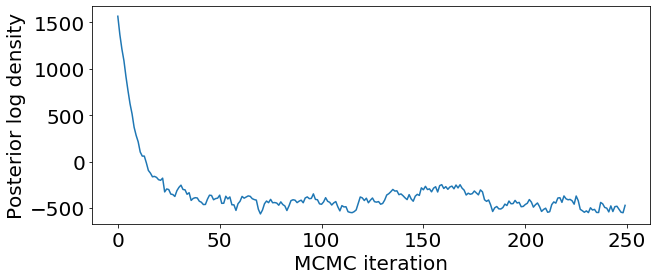
Check convergence by looking at the traceplot for posterior log-density.

plt.figure(figsize=(10, 4))
plt.rcParams['font.size'] = 20

plt.plot(samples['logp'])
plt.xlabel('MCMC iteration')
plt.ylabel('Posterior log density')
plt.show()

Restart MCMC from the last iteration with ‘gibbs_additional_iter()’.

samples, mcmc_info = bridge.gibbs_additional_iter(
    mcmc_info, n_add_iter=250
)

Add more samples (while keeping the previous ones) with ‘merge=True’.

samples, mcmc_info = bridge.gibbs_additional_iter(
    mcmc_info, n_add_iter=750, merge=True, prev_samples=samples
)
coef_samples = samples['coef'][1:, :] # Extract all but the intercept

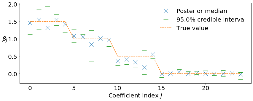
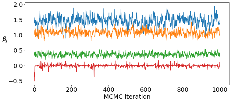
Check mixing of regression coefficients and their posterior marginals.

Typically the convergence is quick and mixing of the regression coefficients is adequate.

plt.figure(figsize=(12, 5))
plt.rcParams['font.size'] = 20

plt.plot(coef_samples[[0, 5, 10, 15], :].T)
plt.xlabel('MCMC iteration')
plt.ylabel(r'$\beta_j$', rotation=0, labelpad=10)
plt.show()

plt.figure(figsize=(14, 5))
plt.rcParams['font.size'] = 20

n_coef_to_plot = 25

mcmc_summarizer.plot_conf_interval(
    coef_samples, conf_level=.95,
    n_coef_to_plot=n_coef_to_plot, marker_scale=1.4
);
plt.plot(
    beta_true[:n_coef_to_plot], '--', color='tab:orange',
    label='True value'
)
plt.xlabel(r'Coefficient index $j$')
plt.ylabel(r'$\beta_j$', rotation=0, labelpad=10)
plt.xticks([0, 5, 10, 15, 20])
plt.legend(frameon=False)

plt.show()